Catherine A. Ball, Erin Battat, Jake K. Byrnes, Peter Carbonetto, Kenneth G. Chahine, Ross E. Curtis, Eyal Elyashiv, Ahna Girshick, Julie M. Granka, Harendra Guturu, Eunjung Han, Ariel Hippen Anderson, Eurie Hong, Amir Kermany, Natalie M. Myres, Keith Noto, Kristin A. Rand, Shiya Song, Yong Wang(in alphabetical order).
1. Introduction
AncestryDNA™ offers several genetic analyses to help customers discover, preserve, and share their family history. Some of the features offered to date are based exclusively on genetic information. These include a genetic ethnicity or ancestry inference (described in Ethnicity Estimate White Paper) and an identity-by-descent (IBD) or DNA matching analysis (Matching White Paper). Other features, like DNA Circles, rely on the integration of pedigree and IBD data across the entire AncestryDNA database (DNA Circles White Paper). Each of these features provides complementary information to a customer: (1) the ethnicity estimate provides a distant picture of a customer’s genetic origins, perhaps hundreds or thousands of years ago; (2) DNA matches provide a customer with a list of fellow AncestryDNA test-takers who are relatives and with whom she or he shares a common ancestor within the last 10 generations; (3) DNA Circles integrate IBD and pedigree data to provide a customer with groups of relatives that appear to share DNA with one another due to a specific shared ancestor, to potentially reinforce their connection to this ancestor. In combination, these features provide a detailed portrait of an individual's genetic ancestry.
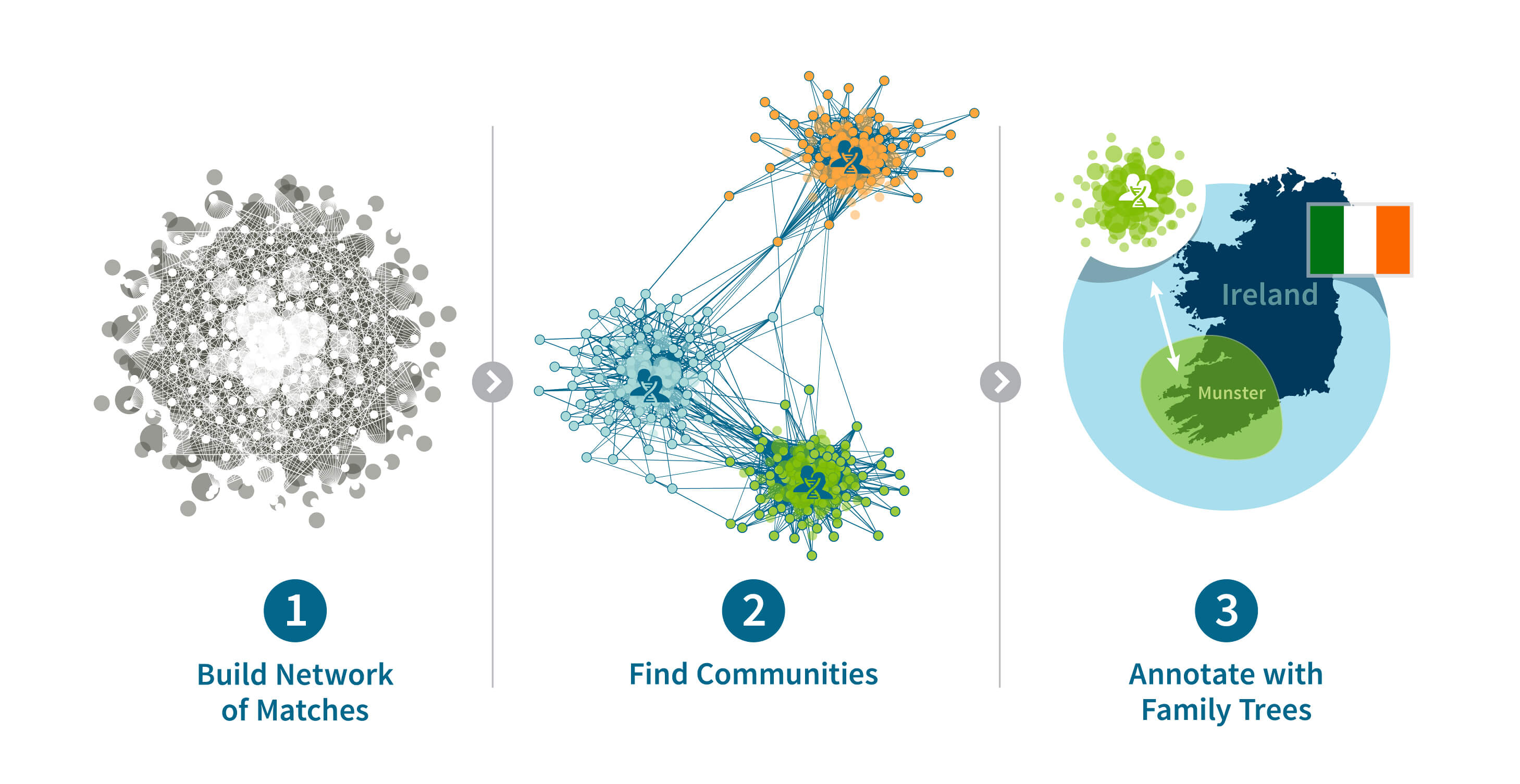
Here, we augment these DNA and pedigree-based insights even further with our new Genetic Communities feature (Figure 1.1). Instead of considering the IBD connection between each pair of customers in isolation, we simultaneously analyze more than 20 billion connections identified among over 2 million AncestryDNA customers as a large genetic network (described below in Section 3). Intuitively, because the estimated IBD connections between individuals are likely due to recent shared ancestry (within the past 10 generations), broader patterns in this large network likely represent recent shared history. The result is that we can identify clusters of living individuals that share large amounts of DNA due to specific, recent shared history. For example, we identify groups of customers that likely descend from immigrants participating in a particular wave of migration (e.g. Irish fleeing the Great Famine), or customers that descend from ancestral populations that have remained in the same geographic location for many generations (e.g. the early settlers of the Appalachian Mountains). Following the identification of these clusters of individuals in the entire network, we can then assign any AncestryDNA customer to one or more of these clusters based on their IBD with other AncestryDNA members. Such assignment can provide a customer with insight into their recent ancestral history, in some cases traceable back to a historical event.
In the following sections, we describe the scientific principles behind the genetic network (Sections 2 and 3), how we identify clusters within it (Sections 4 and 6), our use of DNA and pedigree data to annotate these clusters (Section 5), and finally our method for assigning customer samples to these clusters (Section 7).
2. Population Genetics Motivation for Genetic Communities
In this section, we will discuss some basic population genetics concepts that motivate the identification of Genetic Communities and conclude with an example.
First, we introduce some terminology. An IBD network is a representation of the genetic connections among a collection of AncestryDNA samples. The nodes in such a network are the samples, and the edges between nodes are the IBD connections between samples. We describe the IBD network concept in detail in Section 3. Genetic Communities can be thought of as parts of the network that have a high degree of connectivity—nodes have a higher rate of IBD (and longer IBD) with other nodes inside a given Genetic Community than they do with other nodes outside of it See Section 4 for a broader discussion of Genetic Communities.
To understand why we expect to find Genetic Communities structures in an IBD network, we examine a few basic population genetics principles.
2.1 Genetic Populations
We begin with a discussion around the concept of a genetic population. Numerous definitions of what constitutes a population exist in genetics literature. For clarity, we define a population as a group of people who generally live in close proximity and produce children with one another for multiple generations. This definition is intentionally vague with regards to size and scale. A population can be a large, loosely connected group, such as all Europeans, or it can be a smaller, more closely connected group, such as the Irish. While vague in terms of scale, our definition of a population is specific with regards to time and place. For example, one population might include the ancestors of Europe that lived ten thousand years ago, while another population might include people living in Connecticut 200 years ago.
Each population has a different degree of genetic isolation. When a population has a high degree of genetic isolation, that implies that population members rarely if ever choose to have children with individuals outside the population. On the other hand, a population with a low degree of isolation has high levels of migration and admixture with surrounding populations. Over time, isolated populations develop distinguishable patterns of genetic variation.
New populations can be created in numerous ways. For example, a small subset of individuals from a historical population may migrate to a new location and create a new population that no longer produces offspring with the source population. It is also possible for this new population to separate from the historical population without leaving the source location. Another possibility is for multiple source populations to come together and admix, producing offspring with a mixture of genetic material from formerly separated populations. In all these examples, the unifying feature is the creation of a barrier to gene flow that leads to the development of distinguishing patterns of genetic variation. On the smallest scale, there are many forces including geography, war, religion, culture, politics, and economics that may influence how each of us chooses a mate. What is surprising is that these individual decisions have a significant impact on how genetic material flows through time and space. This raises the question: Can we observe the impact of mate choices made by our ancestors by examining our own DNA? As we see below, we most certainly can.
2.2 An Illustrative Example
Let’s consider a simple example that demonstrates how genetic isolation in a population can lead to Genetic Communities structures in an IBD network.
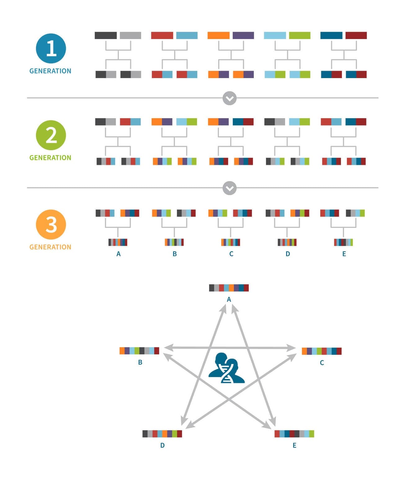
In Figure 2.2, we represent a founding population with 10 unrelated individuals from 10 different populations. Note that the 10 founding individuals do not share long IBD segments of DNA since they are from different populations. In this example, these 10 individuals randomly mate and each of these five couples has two children, creating a second generation of 10 individuals. In this second generation, some individuals are now loosely connected by IBD at the close family level.
We keep repeating this experiment for two more generations; 10 unrelated individuals in the second generation randomly choose mates and each couple has two children, creating a third generation of 10 individuals. Finally, 10 individuals in the third generation randomly mate and each couple has only one child, creating a fourth generation of five individuals.
Interestingly, after these three generations of random mating, all five progeny in the fourth generation have at least one part of their ancestral make up that is shared with each of the other four cousins. These five individuals also have a higher rate of IBD with individuals in this new population than they would with people from the original 10 ancestral populations. In an IBD network made up of individuals from many other populations as well, this particular population would likely form a Genetic Community.
While this example is exaggerated in its simplicity, it helps to illustrate the intuition behind populations and how genetic isolation can create Genetic Communities structures in a large IBD network. Of course, real populations typically have hundreds or thousands of founders and are generally not completely isolated. The degree of admixture (the selection of mating partners from outside the population) and migration in a population will affect the strength of Genetic Communities structures in the IBD network.
It is also important to note that while the IBD network in our example is completely connected in the fourth generation, in large populations we will rarely find a completely connected network. Rather, it is the presence of higher rates of IBD among individuals in the same population due to the intermarriage of hundreds or thousands of families over the course of many generations that creates a modular structure in the network. When this occurs, individuals have more IBD connections to other individuals in the same Genetic Community (or population) than they do to individuals from other Genetic Communities.
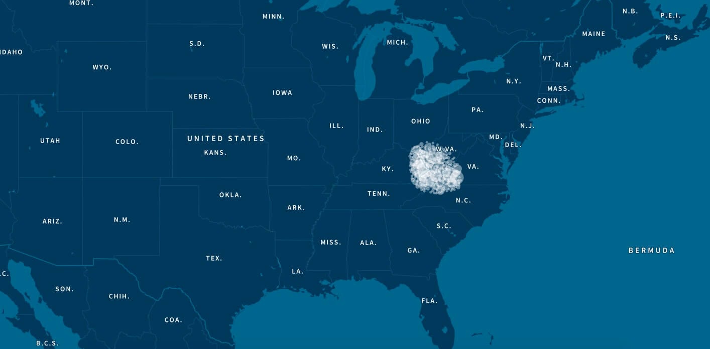
2.3 Example of a Recent Population in the Appalachian Region of Western Virginia and West Virginia
We conclude Section 2 by discussing the creation of a population that settled in western Virginia and West Virginia during the 18th century and use it to provide the intuition that is the basis of our Genetic Communities feature (Figure 2.3).
2.3.1 The History of Western Virginia and West Virginia Settlement
European-American settlement of western Virginia and West Virginia first began in the 1730s, when the Virginia colony promoted settlement of its western mountains to provide a buffer between its established towns and native peoples (Rice 1993). Between 1750 and 1780, the founding population in this region grew. This was a period of peace, prosperity, and aggressive settlement in the Shenandoah Valley following the end of King George’s War in 1748 and a treaty with native peoples in 1752. While the British forbade further settlement with the Proclamation of 1763, Americans pushed into the territory following the Revolutionary War. The construction of roads between 1818 and 1846 promoted further settlement and the isolation of rural areas (Rice 1993). Thus, until the mid-19th century, this region was largely a rural, growing population with settlers who hailed from British, German, or Scotch-Irish backgrounds.
Between 1850 and 1890, this region saw a period of industrialization and a corresponding population boom due to the beginning of the coal industry in West Virginia and the development of the C&O Railroad and coal towns that emerged along its route. For example, Kanawha County experienced a population growth of 700% between 1890 and 1910 (Laidley 1911 [310]). The dawn of the 20th century saw a shift in the pattern with a massive emigration following World War I to the industrial cities of the Midwest and West.
2.3.2 Discussion about Western Virginia and West Virginia Settlement
In this example, we see a new population created in the latter half of the 1700s, consisting of founding individuals from Scotch-Irish, German, and British heritage.
While descendants of this population will surely carry DNA indicating a link to their distant Scotch-Irish, German, and British origins, mating between founders of this new population, and subsequently their descendants over many generations, has resulted in the formation of a new population with patterns of genetic variation that are related to, but distinct from, their historical source populations. The descendants of this new population are people who share large amounts of genetic material with many other descendants in this population. Families intermarried throughout the 1800s until people began to leave after World War I. However, even for the descendants of families that left West Virginia some time ago, the genetic signature persists in the form of long IBD segments shared among descendants regardless of their more recent familial history. Thus, we expect to discover this group of descendants in our AncestryDNA database using the IBD connections between these individuals. In the following sections, we will show how we discover this and other descendant populations in an IBD network.
It is important to note that the examples in this section are intended to illustrate general principles motivating our approach to use community detection to discover Genetic Communities in a large IBD network. These two examples do not represent the unique history of all populations around the world. Each of these Genetic Communities that we discover has its own unique history and degree of genetic isolation and migration. That being said, some of the principles we have discussed will apply in many populations.
3. Constructing an IBD Network from IBD Connections
In this and the subsequent sections, we introduce the methods we use to discover and annotate Genetic Communities.
We begin with the collection of all pairwise IBD connections identified between AncestryDNA customers. A pair of customers is said to have an IBD connection if they share one or more long segments of identical DNA. The most likely explanation for a long segment of identical DNA present in two individuals is that it has been inherited by both individuals from a single common ancestor and thus indicates IBD in the two descendants.
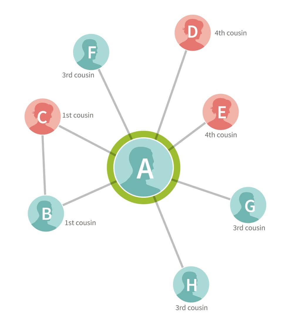
Using Customer A as an example, we have identified, by comparing his DNA with all other customers in our database, seven other customers who have an IBD connection to him (customers B, C, D, E, F, G, and H). (See the Matching White Paper for more details on how we identify IBD connections.) The genetic connections in this small example can be summarized visually by drawing edges between the pairs of people we have identified as connected based on DNA (Figure 3.1). In this particular example, A, B, and C are first cousins, so all three are connected by edges.
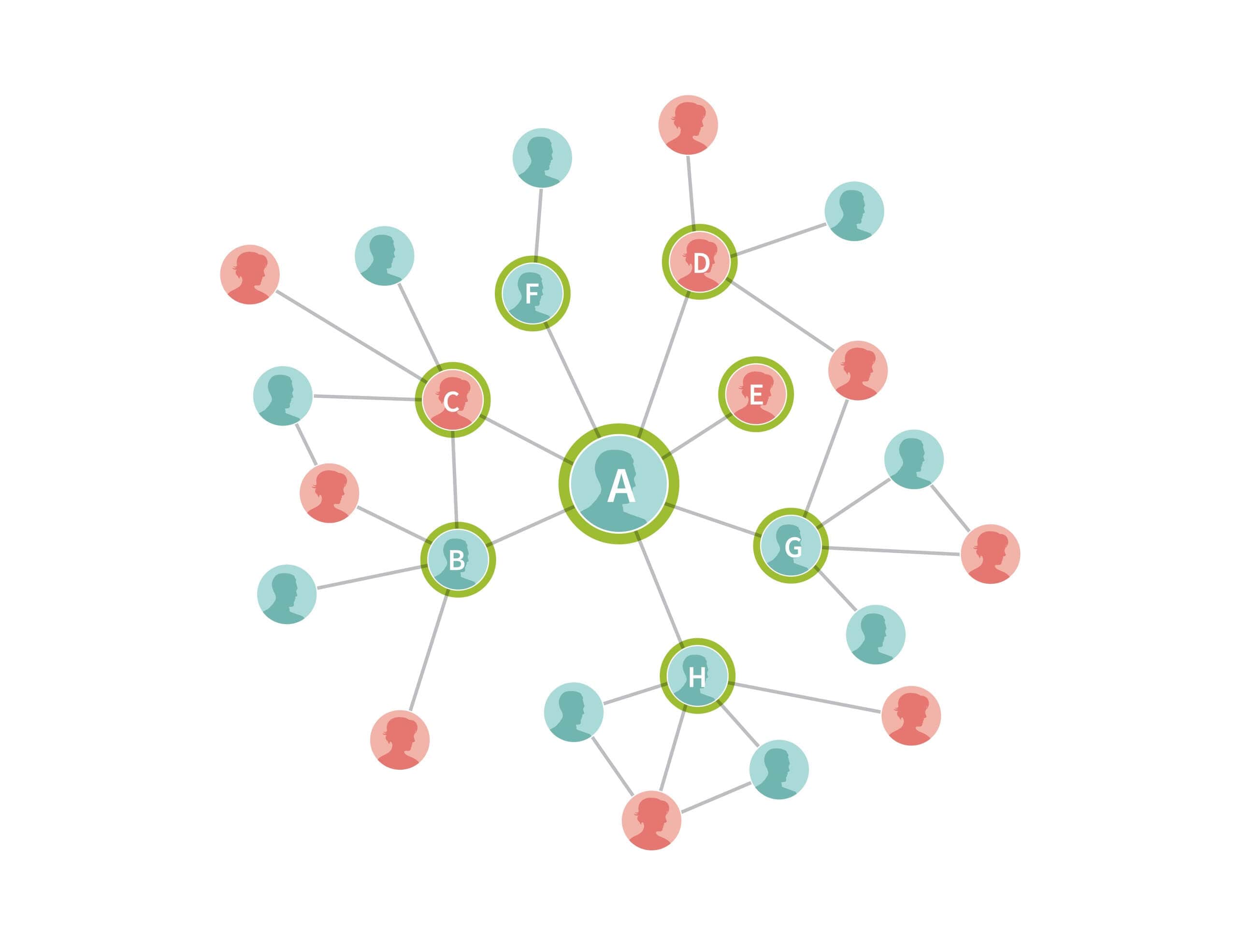
Next, we expand on this example by including the IBD connections found for each of customer A's seven connections (Figure 3.2). The samples that are added in this step are drawn as green circles. The size of the network expands rapidly as we add more people by following the genetic connections between them. In some cases, these new samples are also related to each other, and in other cases these new samples are connected to others that are already included in the network (the blue and white circles). In both cases, we draw edges reflecting the identified IBD connections between these individuals.
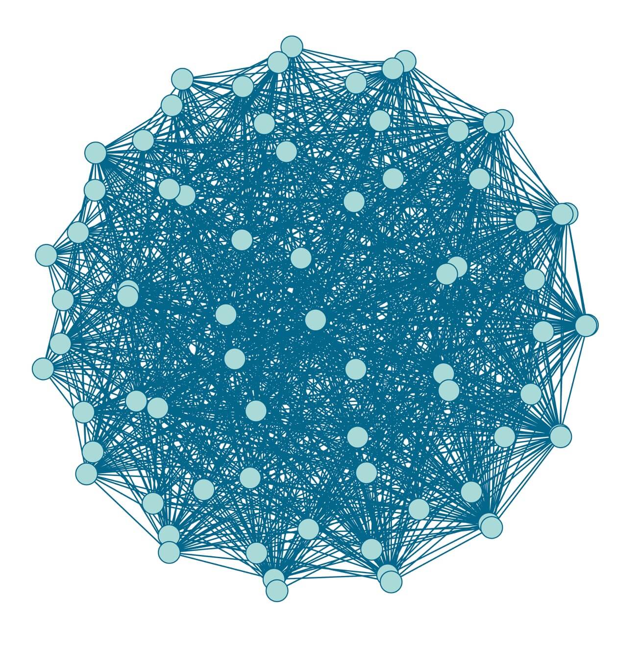
Extending this logic further, we form an IBD network from the IBD connections detected among the millions of individuals that have taken an AncestryDNA test. Clearly, visualizing this network in a single figure, like we have done above, would be difficult. To illustrate what one small part of this network might look like, we show the IBD connections detected between a set of 75 selected AncestryDNA samples (Figure 3.3). This is an example of a particularly well-connected group of samples in the AncestryDNA IBD network, yet there are still pairs of people among this group for whom we did not find an IBD connection.
4. Network Clustering by Community Detection
Given an IBD network, we can subdivide the network into densely connected communities using the Louvain Method—a popular community detection algorithm. Community detection algorithms are network clustering algorithms that identify strongly connected subsets of a network (Blondel et al. 2008, Csardi et al. 2008). In the case of our IBD network, these Genetic Communities represent groups of individuals that are more related to one another than they are to others in the network.
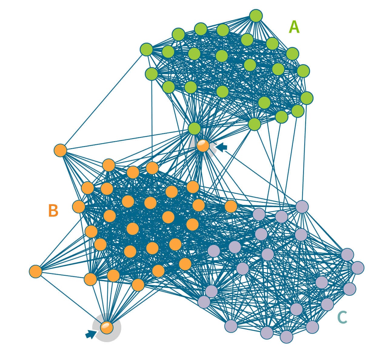
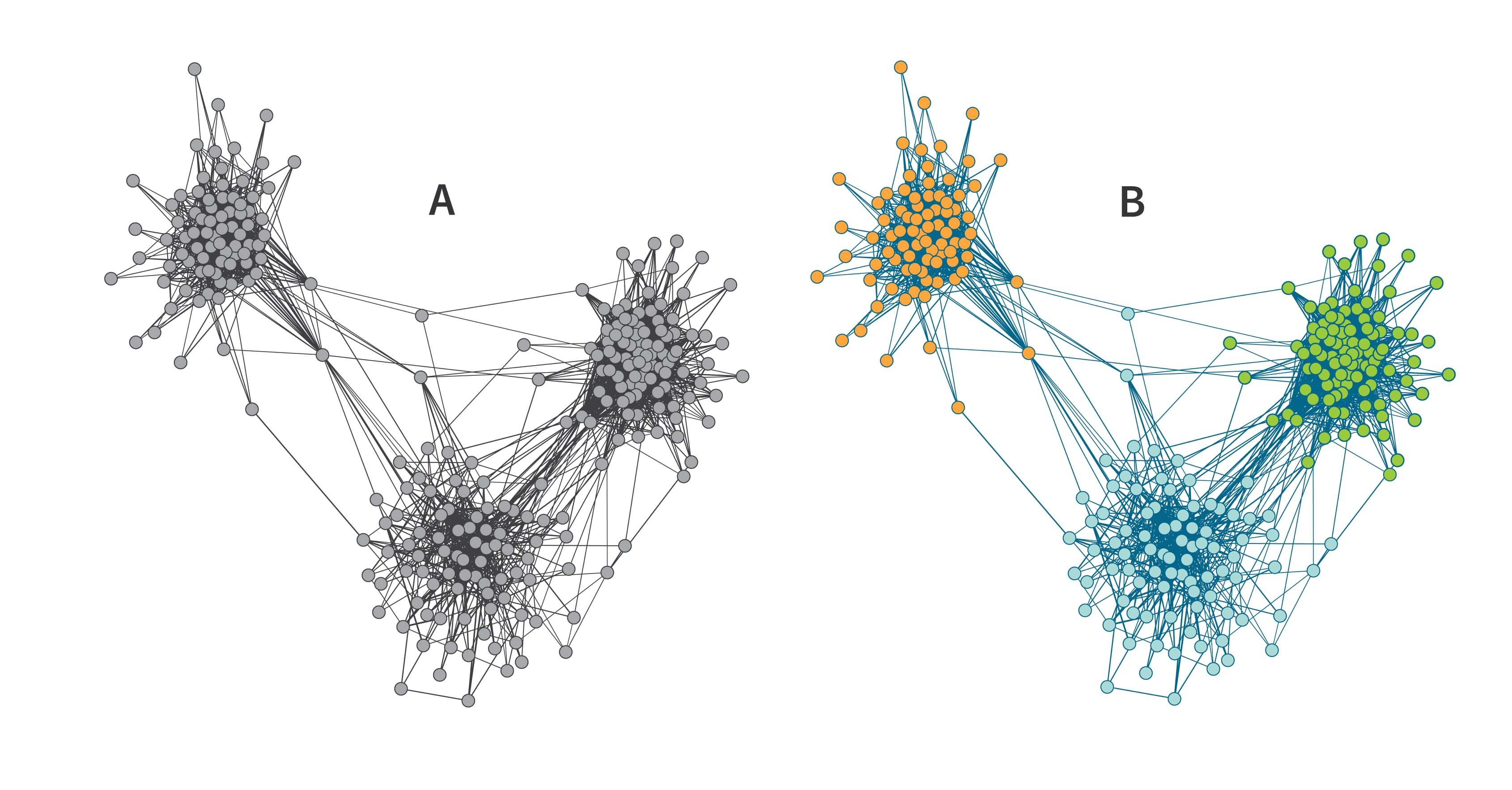
Going back to our visual representation of the IBD network of 75 samples in Figure 3.3, there is no obvious pattern in this IBD network. In Figure 4.1, we present the same network with the nodes rearranged to highlight the structure in the network. In particular, the 75 individuals have been subdivided into three groups, or Genetic Communities, which we have labeled as Genetic Community A (24 individuals, shown as green circles), Genetic Community B (30 individuals, orange) and Genetic Community C (21 individuals, blue). Note that these Genetic Communities were not detected by visual inspection, but rather by running a community detection algorithm on this small IBD network, which assigns each node to one community.
| Genetic Community A (n=24) | Genetic Community B (n=30) | Genetic Community C (n=21) | |
|---|---|---|---|
| Genetic Community A | 276 (100%) | 43 (6%) | 9 (2%) |
| Genetic Community B | 373 (86%) | 163 (26%) | |
| Genetic Community C | 185 (88%) |
Intuitively, the community detection algorithm is subdividing the network into subsets that are more densely connected than the original full network. We can measure how connected a network (or community subset) is using a measure called network density. The density is the number of edges present in the network divided by the number of edges possible in the network. In the case of the IBD network, the network is maximally connected if there is an edge between every pair of individuals. Following community detection in our example above, pairs of individuals within the same Genetic Community are more densely connected to each other than pairs of individuals between communities. For example, 185 edges are contained in Genetic Community C, for a density of 185 × 2 / (20 × 21) = 88%, whereas only 163 edges join members in Genetic Communities B and C, for a density of 163 / (21 × 30) = 26%.
Subdividing this network into three Genetic Communities illustrates another important concept to consider when investigating patterns of IBD connections across many individuals: some individuals have most or all their IBD connections contained within one of the groups, whereas other individuals have IBD connections that spread across multiple groups. An example of the former is a node in the bottom-left corner of Figure 4.1 noted by a blue arrow. The edges emanating from this node all connect to other nodes within the same Genetic Community (Genetic Community B). By contrast, in the middle of the figure, the arrow highlights an individual assigned to Genetic Community B even though this individual has IBD connections with many members of both Genetic Communities A and B, as well as a few with Genetic Community C. Therefore, the degree or strength of membership in a particular group is greater for some individuals than for others.
We divide the AncestryDNA IBD network into densely connected subsets (i.e., Genetic Communities) using a community detection approach. By applying fast network community detection algorithms to the IBD network, we are able to detect population structure within the network. In Section 6, we will discuss how we recursively run community detection to discover fine-scale population structure.
5. Interpreting the Historical and Geographical Characteristics of Genetic Communities
Genetic Communities are discovered solely by using the IBD connections between individuals. As described in Section 2, we expect these connected Genetic Communities to each represent a group of descendants of a particular population. But how can we identify the historical population responsible for a particular set of connections? For this we rely on both genetic data and information present in the pedigrees of descendants of Genetic Communities. In particular, since these connections reflect recent common ancestry, we can look for common features that are shared by individuals in Genetic Communities to correlate the genetic patterns to recent history. These common features help identify a common time, location, or source population from which descendants have ancestry. For example, the people in one of the Genetic Communities might be the descendants of Irish immigrants who came to the United States during the Great Famine in the 19th century.
For this analysis, we rely on two sets of data: (1) ethnicity admixture proportions in 26 global populations estimated from the genotypes (see Ethnicity Estimate White Paper), and (2) pedigrees curated by the users who have taken an AncestryDNA test. The scale and diversity of these data allow us to infer detailed historical and geographic portraits of the Genetic Communities detected in the IBD network.
Before we describe our Genetic Communities annotation process, it is worth noting that our ability to annotate particular Genetic Communities is strongly dependent on the data available. For example, if no members of a Genetic Community have created pedigrees, we have a limited ability to identify a source location for it. It is also important to keep in mind that an individual can only be linked to a particular Genetic Community if they share significant amounts of genetic material with others descending from the Genetic Community. Without a genetic connection, we are not able to link individuals to any of our Genetic Communities. However, the continued growth of the AncestryDNA database is likely to positively impact both of these limitations.
5.1. Average Ethnicity
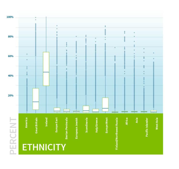
The first feature we look at for each of our Genetic Communities is the genetic ethnicity proportions estimated from DNA. These ethnicity-based annotations can be used to estimate which ancestral populations are overrepresented or underrepresented among individuals from a given Genetic Community. In some cases, Genetic Communities with highly overrepresented ancestral populations can be related to known populations. For example, Genetic Communities corresponding to relatively recent U.S. immigrant groups such as Finnish, Jewish, and Irish people can be identified from the ethnicity-based annotations. On the other hand, Genetic Communities corresponding to groups from New York State, Pennsylvania, and Ohio will have similar, non-distinguishing genetic ethnicity profiles.
Figure 5.1 examines the genetic ethnicity profile of members from a specific Genetic Community discovered through the IBD network. The average ethnicity of these individuals is primarily from Ireland, suggesting that these individuals have shared Irish ancestry.
5.2. Enriched Surnames
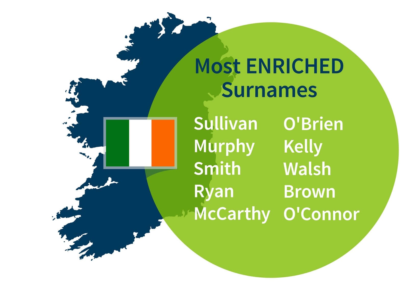
Next, we consider the surnames of the ancestors of Genetic Communities members using aggregated pedigree data. To summarize ancestral surnames for one of our Genetic Communities, we collect all the surnames of recent ancestors associated with the individuals assigned to that Genetic Community. To highlight surnames that are more likely to be characteristic of the Genetic Community, and therefore more likely to yield informative clues about the historical or demographic significance of the Genetic Community, we quantify the statistical evidence (i.e., p-value) that each surname is overrepresented in a given Genetic Community compared to the background surname distribution over all individuals in the full IBD network. Then, we rank the surnames according to the statistical evidence (i.e., smaller p-values), and select the 10 most highly ranked surnames as the surnames that are characteristic to the given Genetic Community. For example, the most highly ranked surnames from the surname annotations associated with individuals assigned to the Irish Genetic Community in Figure 5.1 include “McCarthy,” “Sullivan,” “Murphy,” “O’Brien,” and “O’Connor” (See Figure 5.2).
5.3. Enriched Birth Locations
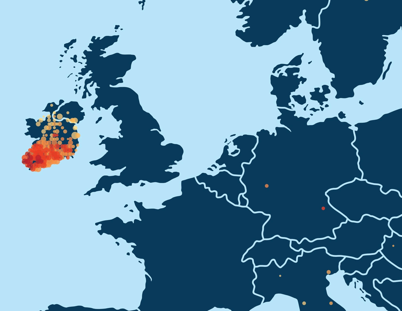
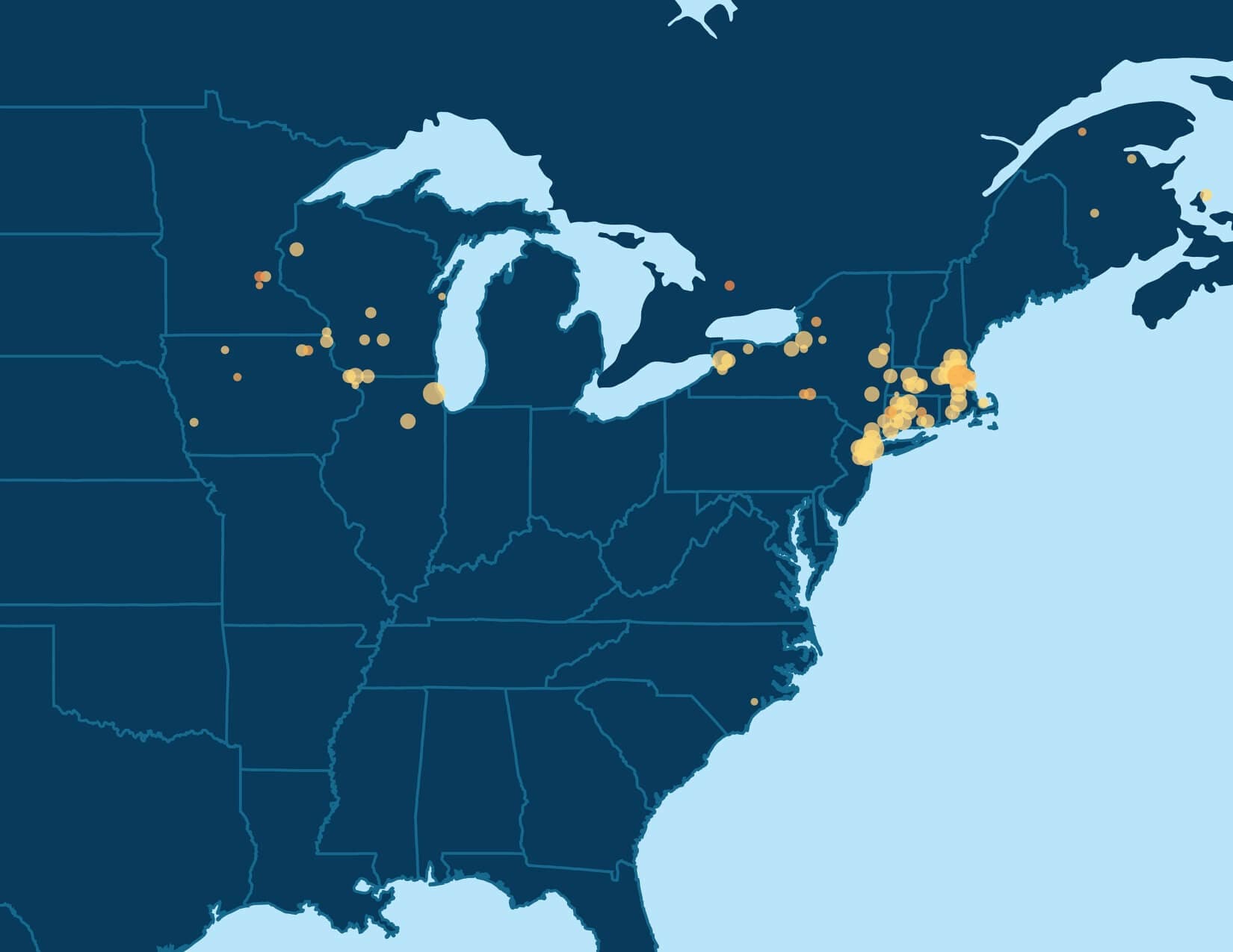
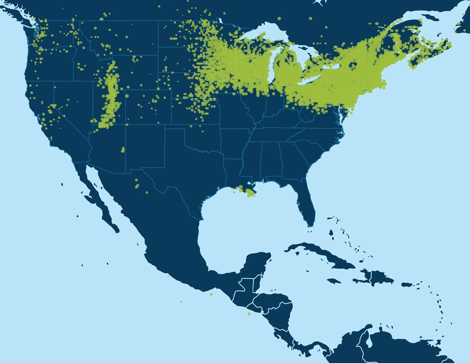
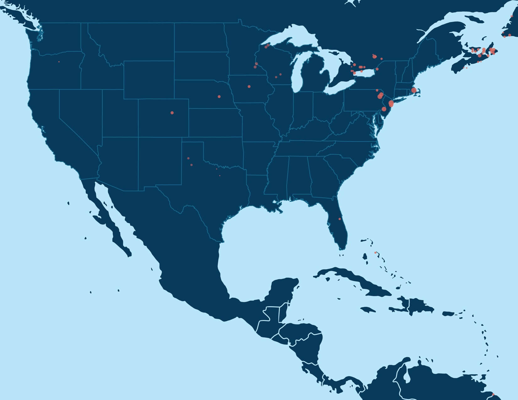
Another type of annotation that we use to characterize Genetic Communities is the birth locations of the ancestors associated with individuals assigned to Genetic Communities. These locations provide useful geographic clues that often can connect Genetic Communities to historical populations. For this analysis, we compile statistics of birth locations of the ancestors specific to Genetic Communities throughout time and summarize the birth location data so that it may be visualized geographically. This is accomplished by converting each birth location, within a specified range of generations, to the nearest coordinate on a two-dimensional (2-D) grid. For each grid point in the 2-D grid, we compute an odds ratio (OR). This OR is defined as the odds that a given grid point of the 2-D grid is associated with the Genetic Community members divided by the odds that the same grid point is associated with users who are not members of the Genetic Community. Using this OR measure, we generate a map that visually depicts grid points in which the largest odds ratios are indicated visually by labels or distinguishable colors. In this way, the highlighted graphical map locations correspond to geographic locations that are disproportionately enriched in a given Genetic Community.
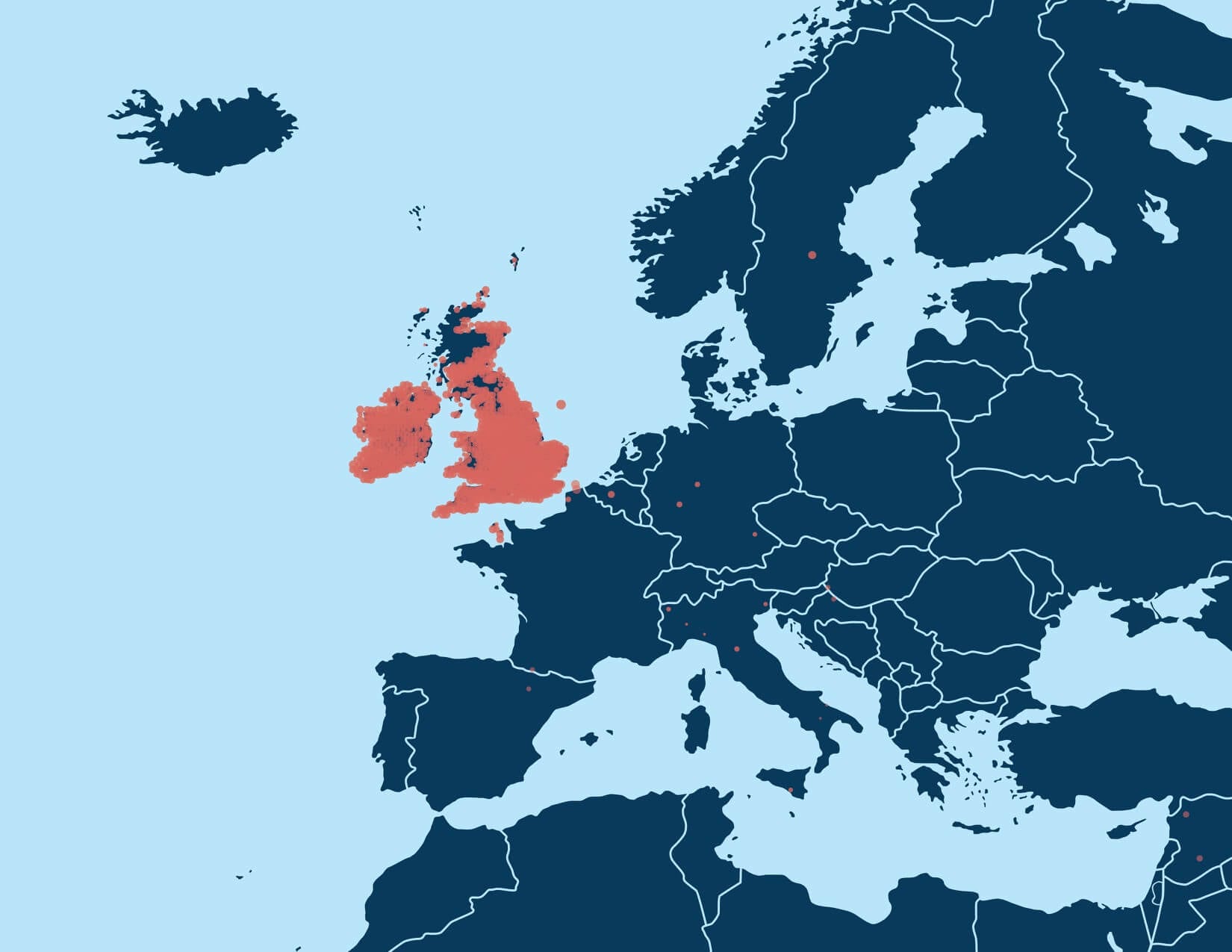
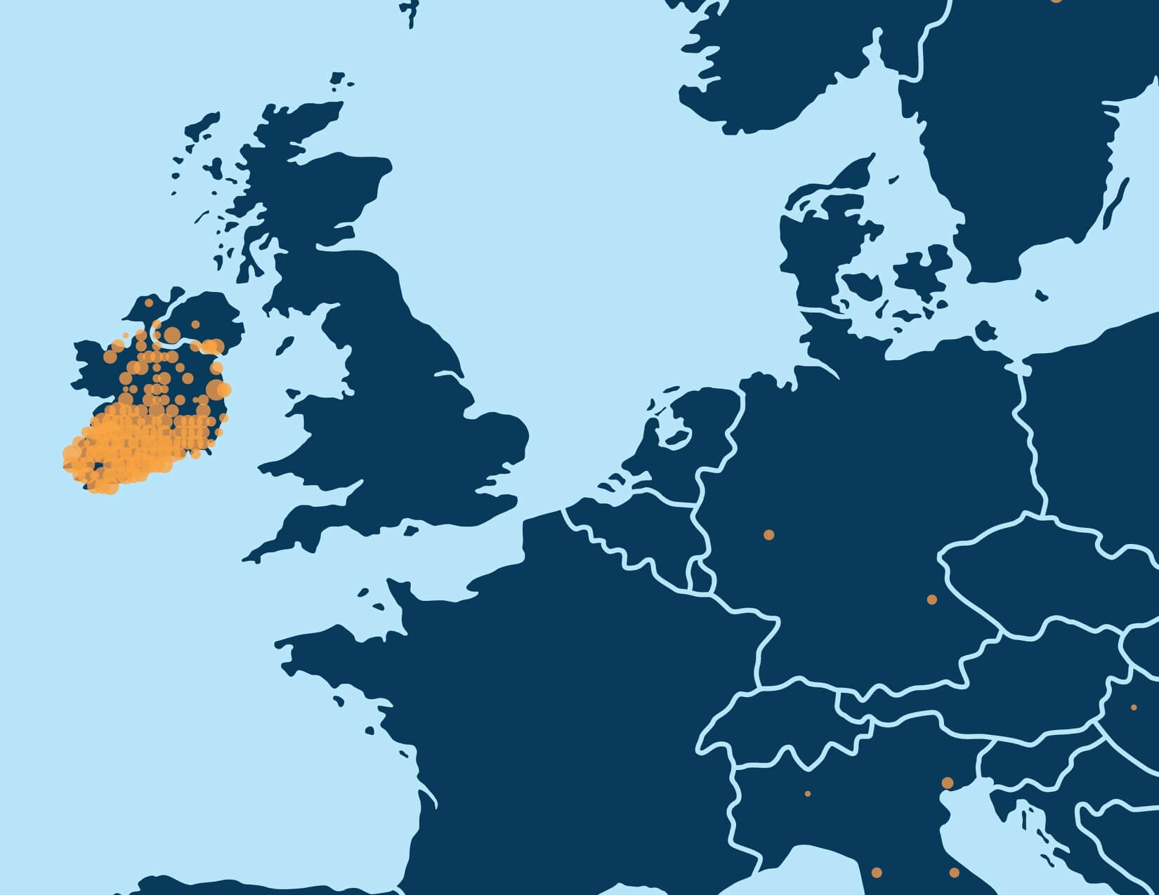
For example, Figure 5.3 shows the enriched birth locations of ancestors born between 1850 and 1910 associated with one of the Genetic Communities with ethnicity from Ireland. This map shows that birth locations with high OR (therefore more enriched) are more highly concentrated in the southern part of Ireland (Munster).
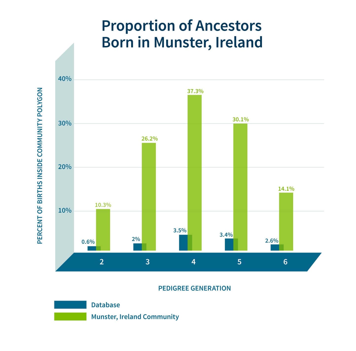
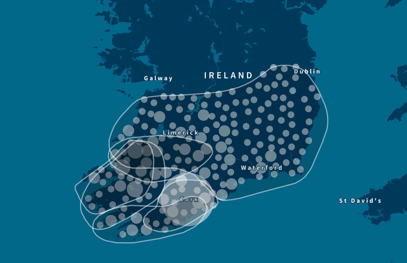
In addition to looking at the odds ratio, we also consider the proportion of the samples in Genetic Communities that have ancestral birth locations in the region identified for each of the Genetic Communities. To do this, we first use the birth location enrichment plots to construct polygons around significant locations specific to each of the Genetic Communities. (These polygons are also used in the product experience). Based on these specific locations, we can determine, for each individual assigned to a Genetic Community, which ancestors were born in this region. For example, in Figure 5.4, we show the proportion of ancestors born in locations inside the Munster, Ireland, polygon by generation. For individuals who are assigned to this Genetic Community, 26.2% of their great-grandparents are born inside the polygon. For individuals not assigned to this Genetic Community, only 2% of their great-grandparents are born in this same location. This analysis supports our interpretation of this Genetic Community as descendants of people who lived in Munster, Ireland.
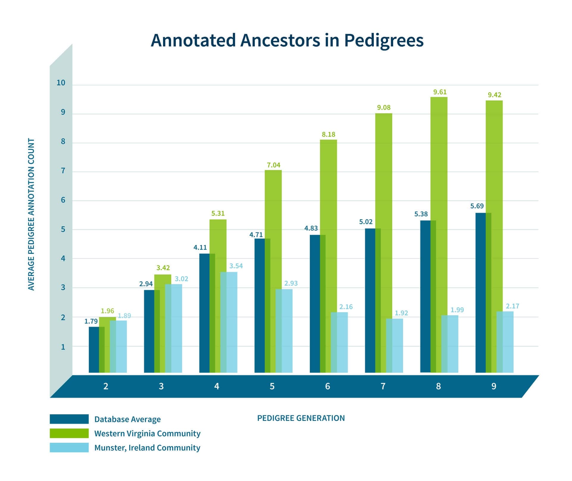
As noted earlier, our confidence in our interpretation of each of the Genetic Communities will depend on the data that has been gathered by the members of the Genetic Community. To assess our interpretation of each of the Genetic Communities, we consider the number of annotations that people have in their pedigrees. For example, people in some Genetic Communities have fewer annotated ancestors at the deeper levels of their pedigrees than others. Two illustrative examples are shown in Figure 5.5—people from western Virginia tend to have many more annotated ancestors at deeper generations than the database average, while the Munster Irish tend to have fewer annotated ancestors at deeper generations. Because of this, we can be more confident in our interpretation of the western Virginia Genetic Community, while we rely on other annotating data when interpreting the Munster Irish Genetic Community. Because there may be many individuals who have not built their pedigrees back into Munster, Ireland, we look at genetic ethnicity. We find that 98% of the individuals assigned to the Genetic Community have >5% Irish ethnicity, thus supporting our hypothesis that these Genetic Community members are from Ireland.
5.4. Migration Patterns
Finally, we also study the migration patterns of the ancestors of members of Genetic Communities through time, as observed from the aggregated pedigree data. We examine how the ancestors of people in Genetic Communities moved from one location to another by looking at the birth locations of parents and children for each generation in each pedigree. Thus, we define a migration path as a path from a birth location of a parent to a birth location of a child.
By looking at changes in these migration paths, we often gain further insight into the population dynamics of the ancestors of the people in Genetic Communities and how those dynamics have changed through time.
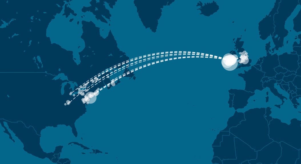
For example, when we look at the Irish Genetic Community from Munster, Ireland, we see a very high frequency of migration paths from Munster to the United States from 1825 to 1875. This time frame corresponds with the migration of 6 million Irish to the United States in the 19th century, which peaked in 1852 during the Irish Famine (Fitzgerald and Lambkin 2008 [8,181]).
5.5 Genetic Communities Interpretation
Based on these four pieces of information—ethnicity, surnames, birth locations, and migration paths—we are often able to infer some of the historical context leading to the strong genetic connections between individuals in the same Genetic Communities. These interpretations are used to guide the names of the Genetic Communities in the user experience, as well as associated historical and other information presented.
6. Recursively Discovering Fine-Scale Genetic Communities
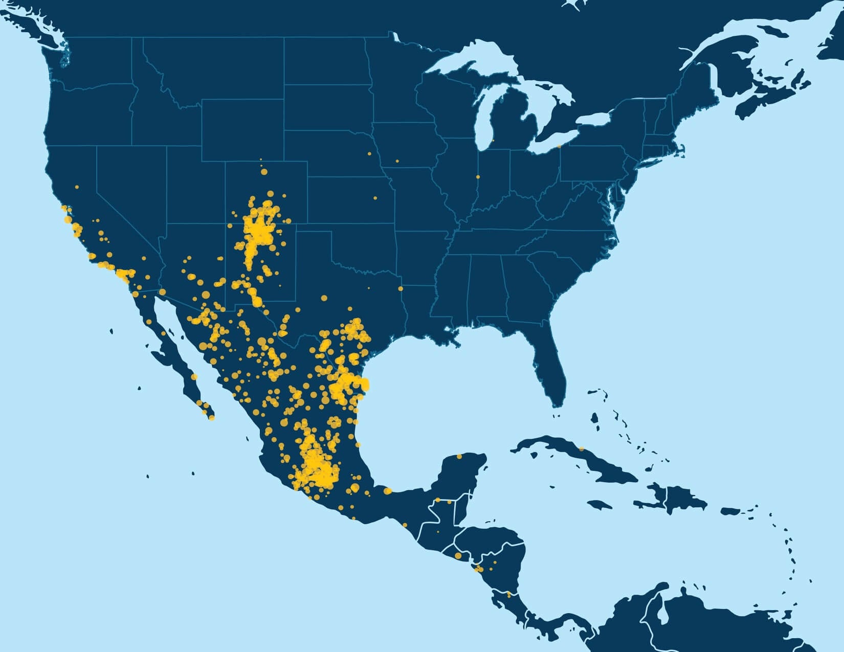
With millions of samples in the AncestryDNA database, recursive execution of community detection enables identification of fine-scale structure in the IBD network. When we first applied community detection to the IBD network of samples in the AncestryDNA database, we initially identified only a handful of Genetic Communities, generally representing either subtle gene flow barriers affecting hundreds of thousands of samples or stronger gene flow barriers separating much smaller subsets of the IBD network. Some examples of more subtle gene flow barriers include Genetic Communities representing people who have ancestors in the northern United States and/or Europe (Figure 6.1A) and individuals of European descent with ancestors in the southern United States. Examples of Genetic Communities due to stronger gene flow barriers include one representing individuals with European Jewish ancestry and another comprised of individuals with ancestry from Mexico and Latin America (Figure 6.1B).

A key discovery of this work is that it is possible to uncover smaller, higher-resolution Genetic Communities through the recursive application of the community detection algorithm. Since each of the observed Genetic Communities is itself a network of IBD connections on which we can apply the same community detection algorithm to discover sub-communities, we performed community detection recursively. Subnetworks, or Genetic Communities from each round, were recursively subjected to an additional rounds of community detection until finer-scale population structures could no longer be stably detected (Figure 6.2).
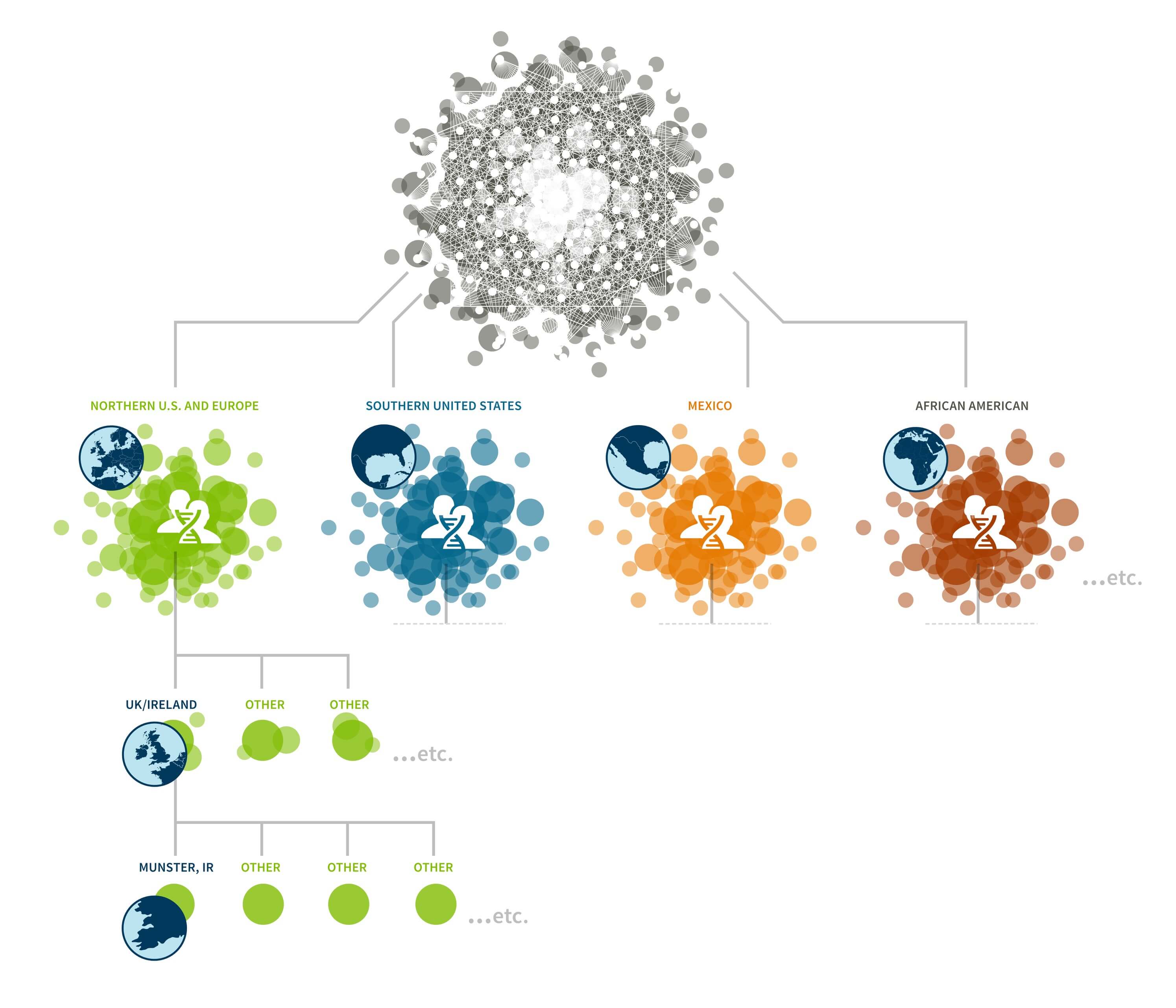
For example, the first round of community detection discovers a large Genetic Community comprised of hundreds of thousands of people with ancestry in the northern United States and/or Europe (Figure 6.1A). Performing community detection solely on this subnetwork reveals several smaller Genetic Communities that correspond to smaller population groups with more specific histories, when the annotating data are considered. We find Genetic Communities representing people with ancestry in Italy, Pennsylvania, New York, or the United Kingdom and Ireland (Figure 6.3).
The Genetic Community visualized in Figure 6.3, discovered with the same algorithm as before, represents a finer population structure than the Genetic Communities we discover from the entire IBD network. We can run community detection once more on this smaller set of individuals. As before, we find a number of Genetic Communities, each corresponding to even finer-scale population structure. We find three Genetic Communities that have ancestors from Ireland (Munster—see Figure 6.4, Ulster, and Connacht), along with Genetic Communities in Newfoundland, Nova Scotia and the United Kingdom.
Once again, we can consider each of these Genetic Communities individually and run community detection again. By running community detection on the Genetic Community corresponding to Munster, Ireland, we find six Genetic Communities corresponding to several (overlapping) regions in Munster (Figure 6.5).
7. Assigning Individuals to Genetic Communities
While the results from the recursive application of the community detection algorithm on the IBD network reveal intriguing fine-scale Genetic Communities, we still require a way to deliver these insights to customers. One possibility is that we select the single Genetic Community that each sample is assigned to at the end of the community detection algorithm and deliver only one Genetic Communities assignment. However, this approach would have two fundamental limitations. First, any single AncestryDNA sample may have strong connections to multiple Genetic Communities. For example, an individual who has shared ancestry with one of the Irish Genetic Communities as well as one of the Italian Genetic Communities may have a strong connection to both, but due to the nature of the community detection algorithm we use, the end result would only deliver an assignment to only one Genetic Community. Second, running community detection daily for a large network with millions of samples and billions of connections is computationally infeasible. Instead we have opted to use machine-learning algorithms, which overcome both of these limitations (Figure 7.1).
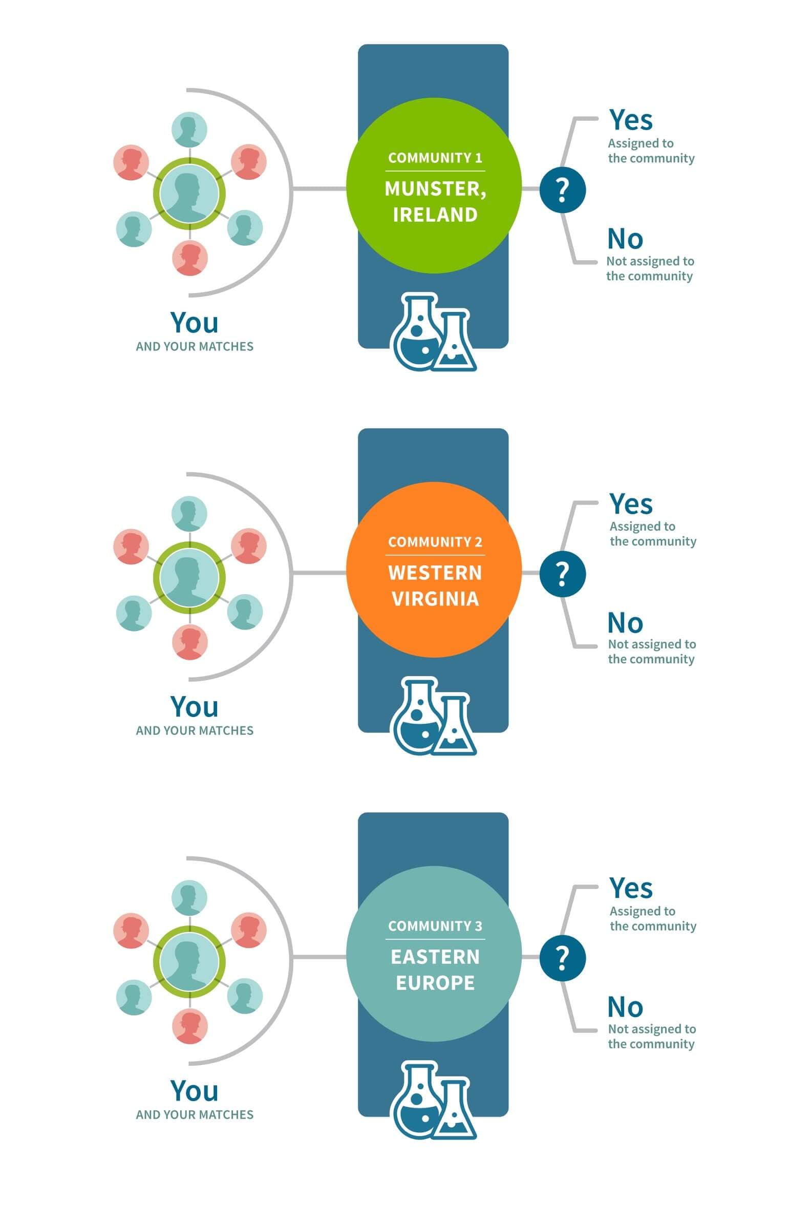
To assign samples to Genetic Communities, we create a reference panel of samples for each of the Genetic Communities that is discovered during recursive community detection. Each reference panel is refined to remove individuals less representative of the Genetic Community and to account for close family relationships. For each reference panel (representing one Genetic Community) that passes certain quality metrics, we construct a binary classifier. Binary classification is a machine-learning approach that assigns a sample to one of two results given a set of features. For example, given features describing a sample’s IBD connection to the network, a classifier will decide “yes, assigned to the Genetic Community,” or “no, not assigned to the Genetic Community.” Since a separate binary classifier is built for each of the Genetic Communities, an individual has the potential to be classified “yes, assigned to the Genetic Community” for multiple Genetic Communities—if they have features representative of those Genetic Communities. For example, an individual with shared ancestry from two Genetic Communities may be assigned to both Genetic Communities. This approach to assigning Genetic Communities can be described as a multi-way classification problem, in which each sample may be classified into zero, one, or more Genetic Communities (Figure 7.2). Using this multi-way classification scheme, we are able to assign individuals to many Genetic Communities and sidestep the infeasibility of running community detection on the full AncestryDNA database with each new sample.
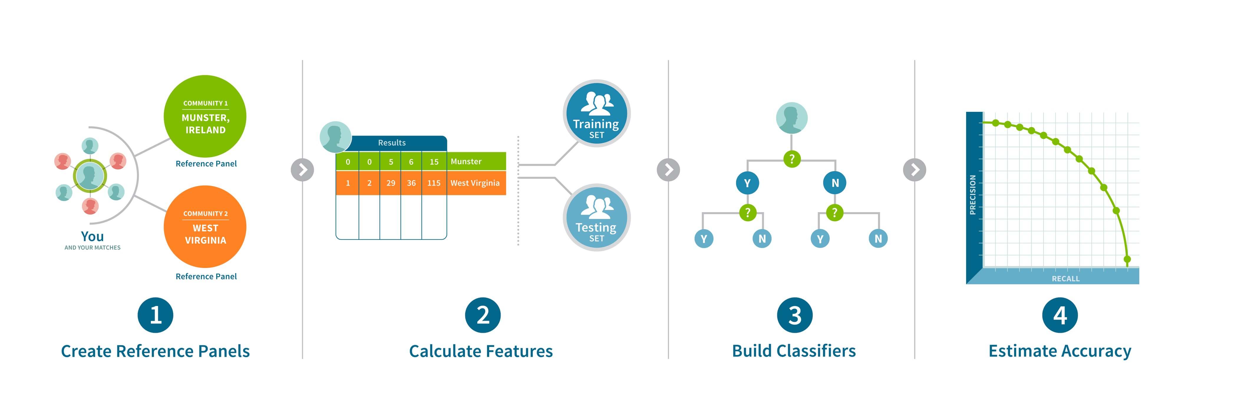
The features that are used in these classifiers are found by summarizing each sample’s IBD connections in the IBD network and its discovered Genetic Communities. Because not every generated feature is useful for each classifier, we use standard feature selection techniques to select only the most informative features for each model. The number of selected features varies for each classification model.
For each of the Genetic Communities, we use the selected features to train a binary classifier that can be saved and used to assign any AncestryDNA sample to zero, one, or more relevant Genetic Communities. We use a validation set (a set of samples that were clustered into a Genetic Community, none of which were used for training) to estimate the accuracy of each classifier and can therefore qualify each "yes, assigned to the Genetic Community" classification with a confidence, that we divide into categories as shown in Table 7.1.
| Confidence Level | Validation Set Accuracy |
|---|---|
| Very High Connection | Classifications with about 95% accuracy on the validation set |
| High Connection | Classifications with about 80% accuracy on the validation set |
| Moderate Connection | Classifications with about 60% accuracy on the validation set |
| Low Connection | Classifications with about 40% accuracy on the validation set |
| Very Low Connection | Classifications with about 20% accuracy on the validation set |
For ease of communication, these confidence levels are condensed and displayed to customers in the following three groups:
- Very High Connection: Very Likely
- High and Moderate Connection: Likely
- Low and Very Low Connection: Possible
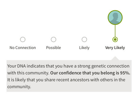
We present the results to the customer in the product experience that you see today (Figure 7.3).
8. Conclusion
In this white paper, we describe our identification of, and assignment of individuals to, Genetic Communities. These Genetic Communities correspond to fine-scale population structure due to very recent, and sometimes documented, historical patterns.
First, we identify genetic connections defined by sharing a recent common ancestor, or IBD, among millions of AncestryDNA samples. When these connections are aggregated into a network, our computational methods reveal densely connected clusters (genetic communities) in which the members of each cluster are more related to each other than to members of other communities. Next, using genetic ethnicities and user-generated pedigrees, we annotate these genetic communities to identify the putative historical origins of such population substructures, and to infer temporal and geographic patterns of migration and settlement. Finally, by applying machine-learning techniques, we infer membership of AncestryDNA samples to these genetic communities, thus providing a detailed survey of their contemporary family history in North America, Europe, and elsewhere.
As the AncestryDNA database continues to grow, we expect that our ability to discover additional structures in the IBD network will be enhanced. This will likely lead to discoveries of genetic communities in new areas of the world and with further granularity, leading to a richer family history experience for AncestryDNA customers.
9. References
Blondel, Vincent D., Jean-Loup Guillaume, Renaud Lambiotte, and Etienne Lefebvre. "Fast Unfolding of Communities in Large Networks." Journal of Statistical Mechanics 2008, no. 10 (2008). doi:10.1088/1742-5468/2008/10/p10008.
Csárdi, Gábor, and Tamás Nepusz. "The Igraph Software Package for Complex Network Research." InterJournal Complex Systems 1695 (2006).
Fitzgerald, Patrick, and Brian Lambkin. Migration in Irish History, 1607–2007. Basingstoke: Palgrave Macmillan, 2008.
Laidley, W. S. History of Charleston and Kanawha County, West Virginia and Representative Citizens. Chicago: Richmond-Arnold Publishing, 1911.
Rice, Otis K. West Virginia: A History. Lexington, KY: University of Kentucky, 1985. Accessed May 13, 2015. https://muse.jhu.edu/.